Cul-de-Sac Design with Alignment as a Reference Feature
Updated February 11, 2023
This article applies to:
- RoadEng Civil
- RoadEng Forestry
Cul de Sac Design Using an Alignment as a Reference Feature
Note: you can download the files here: Files.zip
This example shows how to design a cul de sac in the Location module. Reference features can be used to control the cross-section templates and display intersected and projected features in section and profile. In this case, we are using the Center Line (CL) feature of an additional horizontal alignment.
Drawing the cul de sac outline can be done in several ways:
- with the mouse (easy but not accurate, but you can measure and adjust)
- by coordinates
- by azimuth and distance, as shown in this example (easier than coordinates and independent of projection)
Open the Location module. Open stage_1.dsnx file (included with this example). The screen should display the initial section of the Road alignment as shown in Figure 1.
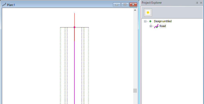
Figure 1: Road Alignment
Use the Project Explorer to create a New horizontal alignment. Change its name to Cul de Sac.

Figure 2: New Horizontal Alignment Cul de Sac
Browse for the topo.tex file included in this example.
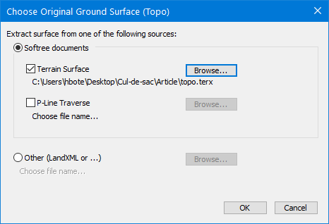
Figure 3: Original Ground Surface: topo.terx
For the Initial Alignment, set the coordinates of the initial point (IP 1): X = 161.00, Y = 220.50
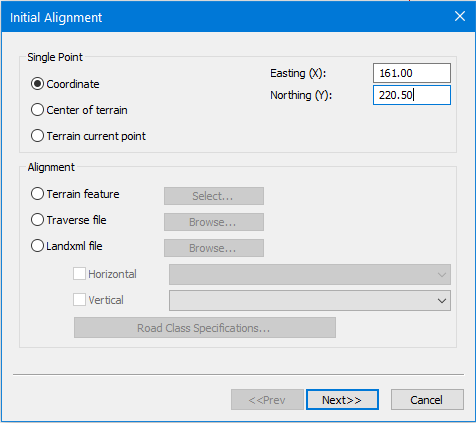
Figure 4: Coordinates of the Initial Point IP 1
Choose Empty for the Initial Cross Section Template. We are using the CL of the Cul de Sac alignment.

Figure 5: Cross Section Template
Your Plan view should be like the figure below:
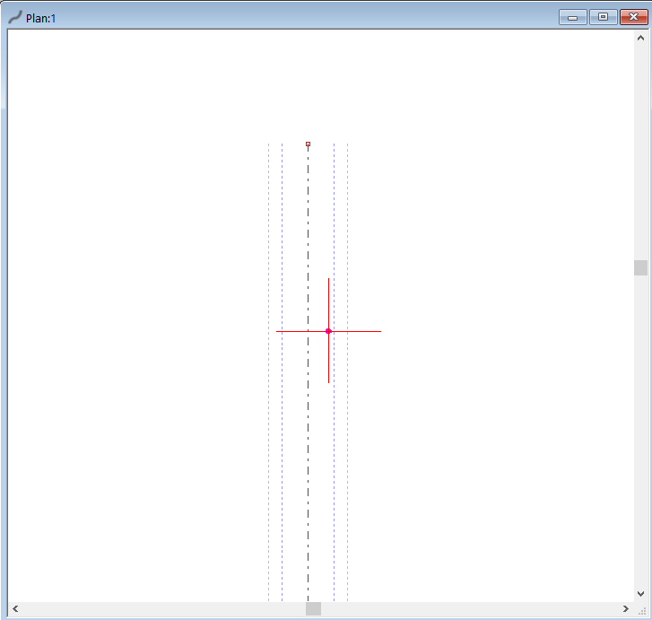
Figure 6: Initial Point (PI 1) of the Cul de Sac Alignment
In the Horizontal Curves panel, use the ![]() button to add the next IP (IP 2): Azimuth = 00.00, Horizontal Distance = 27.98.
button to add the next IP (IP 2): Azimuth = 00.00, Horizontal Distance = 27.98.
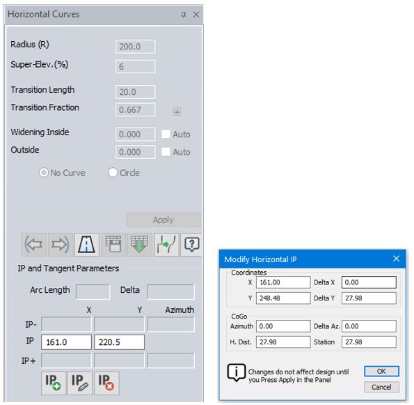
Figure 7: Second Point (PI 2) of the Cul de Sac Alignment
Add the remaining IPs with the values shown in the table below.

The result should be similar to the figure below (figure 8):
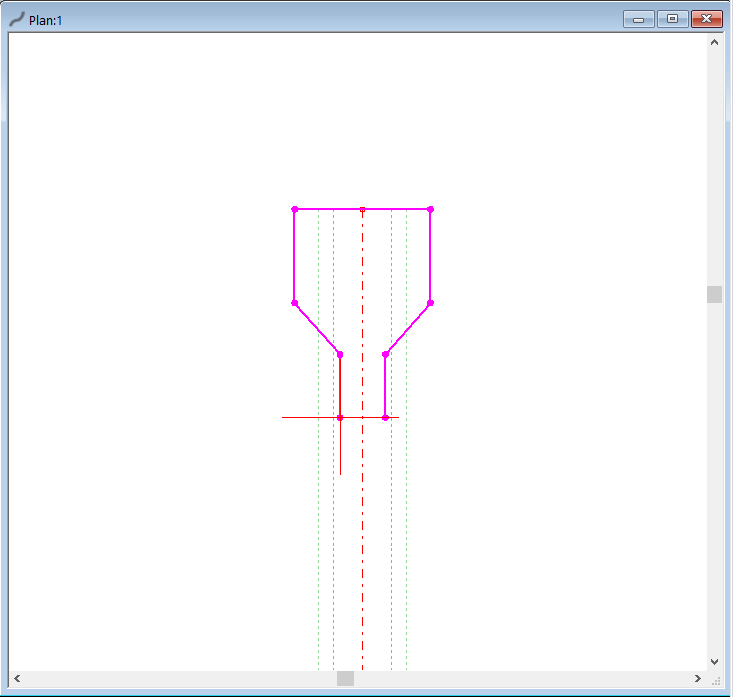
Figure 8: Tangents of the the Cul de Sac Alignment
Apply 50m-radius curves to IPs 2 and 7. For IPs 3 to 6 apply 30m-radius curves.
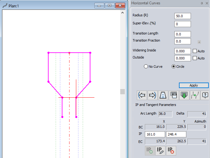
Figure 9: Adding Curves to the IPs
On the Plan view, enable labels (BC/EC, Horiz. IPs at Curves). You screen should be like the figure below.

Figure 10: Center Line of Cul de Sac Alignment (with Labels)
Create a Reference Feature (CL of Cul de Sac Alignment).
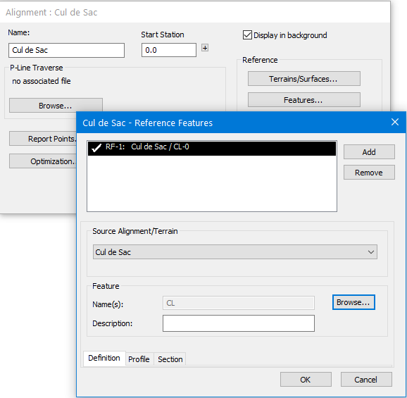
Figure 11: Feature CL-0 as Reference Feature
On the Road alignment, use the Template Editor to set the AcpWidth (Rural I template) to REF-1 Cul de Sac CL-0
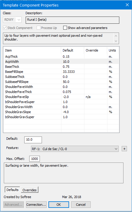
Figure 12: Setting AcpWidth to Reference Feature RF-1
On Plan view, set the Report Points Auto Interval to 0.5m.
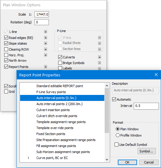
Figure 13: Setting AcpWidth to Reference Feature RF-1
Optionally, you can configure the 3D Window to add a Corridor Surface (Final Grade Surface).

Figure 14: Cul de Sac in Plan and 3D View