External Movement
Updated November 17, 2021
This article applies to:
- Softree Optimal
In this example, we consider the most common applications of external material movement. In the first part, we will look at overflow/underflow reporting and how to configure the reporting area in the Alignment Panel. In the second section, we will examine side-cast and how to add range based constraints.
- If you are starting here, open the Softree Optimal
 application. If you are continuing from the previous start at step 4.
 - File button | Open. Select Hart Rd.dsnx. Press Open.
- Arrange your screen as before, to look like the Figure 2. You may need to arrange your visible windows by selecting the View tab | Tile Vertically

- Press the Options button
 in Alignment Properties Panel toolbar.
- Select the Pits tab.
- Select Pit2: Borrow variable stn: 0.00.
The Pits dialogue (below) is used to create and configure borrow and waste sites for volume handling. We will discuss the options briefly before we continue the exercise.

Figure 1: Pits tab in the Optimization Options dialogue box.
The controls at the top of the dialogue box allow you to specify four types of pit:
| Borrow (variable) | Material can be extracted from the pit if necessary. |
|---|---|
| Borrow (not variable) | The quantity specified must be removed from the pit. |
| Waste (variable) | Material can be dumped in this pit if necessary. |
| Waste (not variable) | The quantity specified must be placed in the pit: stockpile. |
Note: We sometimes refer to variable pits as smart pits. And pits that are not variable can be referred to as fixed pits or stockpiles.
In earlier versions of RoadEng, there was no such thing as a variable pit; when you open older documents, borrow/waste assignments will be converted to fixed pits.
A brief description of the other pit attributes follows.
|
Access station - location on the alignment from which the pit is accessed. Access Distance - from access station to the borrow/waste site (sometimes called dead-haul distance). Comment – for tracking purposes (optional). Waste quality – The minimum material quality required (non-variable only). Material - available (borrow pit only). Excavation $ - Cost to excavate (borrow pit only). Capacity limit - Maximum volume of borrow or waste (variable only). Volume - Exact amount of borrow or waste (non-variable only). |
|

Figure 2: Pit Attributes
Overflow and Underflow
- In this design, material is balanced by use of both borrow and waste pits. The quantities can be displayed in output reports and in the Optimal Haul Diagram (discussed later).
Let’s see what happens when we remove the only waste pit:
- Select Pit-1 (Waste variable) then press the Remove button.
- Press OK, to close the Options dialogue box.
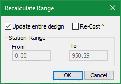
Figure 3: Recalculate Range dialogue box.
- Press OK to recalculate cross sections.
Now let’s update the costs explicitly (Recalculate Range, above, can do this also, but it doesn’t report warnings).
- Press the Re-Cost^ button in the middle of the Alignment Properites panel to open the dialogue box.
- Press the Calculate button inside the dialogue box.
Because it was impossible to balance materials, you will be presented with the log shown below. The Log shows an overflow of 4,861 cu. m. of excavated material.

Figure 4: Log for Cost Calculation information popup when balance issues encountered.
- Press OK to close the log.
Note: The most recent log text is always available in the Log tab of the Vertical Optimization Options dialogue box.
Configuring the Alignment Panel reporting area
Overflow/Underflow information can also be displayed in the configurable reporting area.
- Add Overflow and Underflow to the displayed items:
- Click on the Options button
 at the top of the panel (or right click in the reporting area and choose menu Choose fields to report) to open the Optimization Data Report dialogue box.
 - Open
 the Volume branch in the Available list the select and Add both Overflow and Underflow to the Selected list (as in the figure below).
 - Press OK to close and save changes.
The information area (shown below right), now displays these values whenever they are available.


Figure 5: Configuring the information area to show Overflow/Underflow values.
The Overflow field in the reporting area indicates an excess of material; this is because there is no waste pit available. This is referred to as Overflow to distinguish it from ordinary pit waste. When necessary, an overflow pit is created at the start of the alignment. Note that the cost is the same because the waste pit we removed (previous steps, above) was also located at the start of the alignment.
- Next, use the same procedure to remove Pit-2 (Borrow variable) Rock Pit and then Re-cost.
![]()
Figure 6: After rock borrow pit removal, Underflow is no longer zero.
The Underflow field in the Reporting Area now indicates a shortage of material. This is referred to as Underflow to distinguish it from ordinary borrow. When necessary, an underflow pit is created at the start of the alignment. Note that the cost is different now for two reasons:
- Haul costs are different because the underflow pit is not at the same location as the original borrow pit.
- Excavation costs are also different. The cost of material from the underflow pit is determined from the ground type table ($20.00/cu. m); the original borrow pit had an explicit unit cost of $6.00/cu. m.
You may have also noticed that the Mass Haul diagram changed during this process.
Note: Overflow and Underflow is not shown in the Mass Haul diagram.
Finally, there is a small change in the Overflow volume (and totals); this is caused by a slightly different sample set used in the optimal haul calculation. When there was a pit located at station 450, there were also a pair of automatic report points at stations 449.9 and 450.1; these report points have been removed and the volume is slightly different.
Material quality application
At first glance this may seem strange; how can there be an excess and a shortage at the same time? If you look carefully at the design, you will see that the designer has specified SR (rock) fill for a portion of the road (menu Edit | Assign Parameters by Range, Fill Types tab). However, most of the material being excavated along the alignment is GR (as defined in the Sub-Horizons tab of the same dialog box). Because GR has a lower quality than SR (as defined in our Ground Types table, see Figure 3‑7: Cost Parameters), it cannot be substituted for the required SR fill.
In summary, we are short of rock fill but we have an excess of gravel excavated from the roadway.
Sidecast of material
Sidecast provides an alternative to using a waste pit; material is discarded along the corridor beside the road.
- Open the Options dialogue box, select the Constraints tab, and then the Sidecast tab.
We have an excess of about 5000 Cu. m of material; the length of the alignment is 950m; this works out to about 5 Cu. m/m. If we could discard this much material along the side of the constructed road, we would no longer have to haul material to a waste pit.
- Setup for Sidecast, as shown in the figure below:
- Check the Active checkbox.
- Enter a Linear sidecast of 5.0.
- Leave the station range as is (“..” to “..” represents the whole road). But note that you can define station ranges if desired.
- Press Add/Edit (warning – it is easy to forget this step!).
- OK to close Options dialogue box.
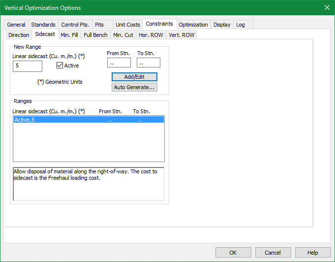
Figure 7: Sidecast Constraints
- Re-Cost^ the design.
The overflow volume has changed, Softree Optimal returns with an overflow of 2166 Cu. m.
- Use the procedure described in step 9 above to add Sidecast volume to the reported items.

Figure 8: Sidecast volume displayed in the reporting area
Why is the Sidecast so much smaller than what we calculated? Sidecast is only practical where excavation is occurring so the actual station range where sidecast is occurring is less than the length of the alignment. We need to choose a value bigger than 5.0 to get rid of all of our excess cut.
- Repeat the steps above using a Linear sidecast of 10.0. Then Re-Cost^.
Observe that the volume of overflow has been reduced significantly. Similar to pit volumes, sidecast quantities can be displayed in output reports and in the Optimal Haul Diagram (discussed later).
16. File button | Exit. Do not save changes.